Skip to content

Blog

N + 1 Devices

cuDF-Polars can scale a familiar Polars query across multiple GPUs with only a few configuration changes

With cuDF-Polars 26.06, we have a new execution backend: RapidsMPF. RapidsMPF handles both execution and the distributed collectives needed for multi-GPU, out-of-core algorithms. That's a lot of verbiage. More simply, RapidsMPF gives cuDF-Polars a way to coordinate work and move data across workers/devices/ranks/etc.

In this post I want to start exploring the multi-GPU capabilities of cuDF-Polars.

When searching for more performance, more memory, more of anything, we often go to plaid -- wait, not plaid -- distributed. Well, sometimes distributed -- multiple GPUs, or multiple CPUs, or nodes, or clusters...but what we are really trying to get at is parallelism (not concurrency): how to run mulitple tasks at the same time.

Learning to use multiple devices may seem intimidating. N+1 of anything is often perceived as an advanced feature, or at least an intermediate one. But our hardware and software keep changing and we can find examples (perhaps even models) of excellence which offer parallelism wiht little to no visibility to the enduser. NumPy is one such example where multi-threaded execution is now avaiable without any effort or input from user. That's probably the decades of labor in underlying libraries like LAPACK/BLAS, a bunch of magic linking and packaging, and perhaps most importantly, thoughtful API design.

The GPU analytics world is still a somewhat nascent adventure, and we collectively are exploring how to deliver speed-of-light performance and ease of use without requiring extreme levels of expertise. For these reasons, the multi-GPU experience is typically opt-in and the user should be more cognizant of what they are opting into. Still, many libraries (PyTorch, XGBoost, HugginFace) including cuDF-Polars are actively exploring *and shipping• solutions which enable multi-GPU capabilities without requiring in-depth knowledge of GPU hardware or software.

With that said, if you find yourself on a single-node multi-GPU (SNMG) machine, you CAN leverage all this hardware with just a few additional engine configurations to otherwise standard Polars code. Recall that the out-of-box experience for most cuDF-Polars users is a single parameter change: collect(engine='gpu'). Now we just need to take the advanced step and define a multi-GPU engine explicitly:

from cudf_polars.engine.ray import RayEngine

engine =  RayEngine()
result = (
    pl.scan_parquet("/data/*.parquet")
        .filter(pl.col("amount") > 100)
        .group_by("customer_id")
        .agg(pl.col("amount").sum())
        .collect(engine=engine)
    )

Hmmm, actually, not too bad. In fact, it's quite simple! The above will automatically start using all the GPUs in the same box. It even comes in ContextManager form for easy cleanup:

from cudf_polars.engine.ray import RayEngine

with RayEngine() as engine:
    result = (
        pl.scan_parquet("/data/*.parquet")
          .filter(pl.col("amount") > 100)
          .group_by("customer_id")
          .agg(pl.col("amount").sum())
          .collect(engine=engine)
    )

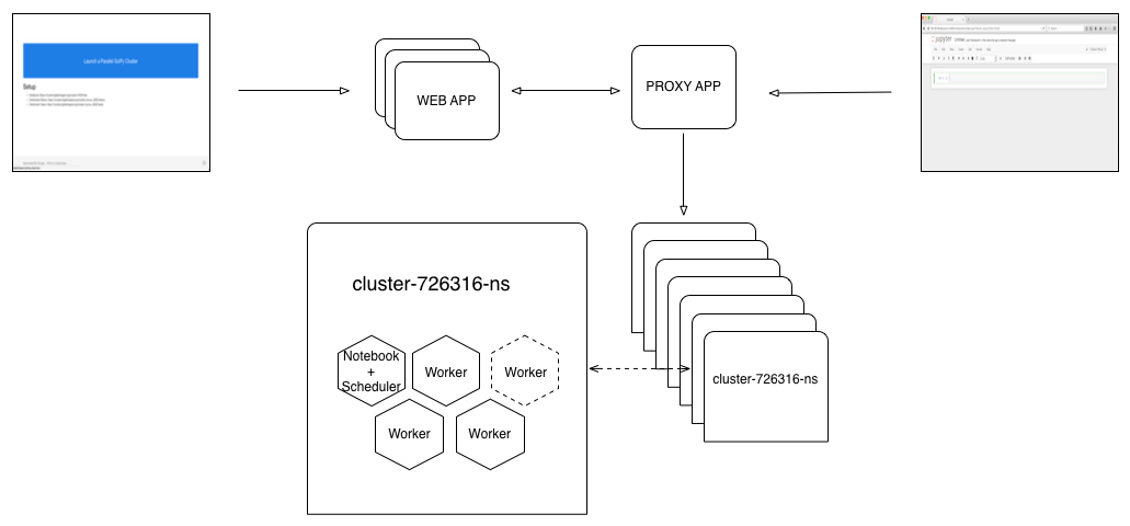
This will automatically start one ray worker per GPU, and cuDF-Polars (RapidsMPF) will execute all the work evenly across each device. There is no scheduler here, for those familiar with task-based systems like Spark. Instead, all workers will get the same execution graph (a physical plan) and operate independently. Synchronization points are inserted into the physical plan where communication is required: groupby-aggregations, join/merges, etc. These higher level operations are composed of RapidsMPF atomic collectives common in distributed computing: shuffle (all-to-all), allgather, allreduce, sparse-all-to-all, etc. For now, let's stay above these details and continue exploring what kind of options are available to us.

I was able to get some time on a machine with 4 T4s. These are older and a bit smaller compared to more contemporary devices -- only 16GBs of VRAM/GPU -- but with four we have a whopping 64GBs!

$ nvidia-smi
Tue Jun 16 16:59:53 2026
+-----------------------------------------------------------------------------------------+
| NVIDIA-SMI 580.159.04             Driver Version: 580.159.04     CUDA Version: 13.0     |
+-----------------------------------------+------------------------+----------------------+
| GPU  Name                 Persistence-M | Bus-Id          Disp.A | Volatile Uncorr. ECC |
| Fan  Temp   Perf          Pwr:Usage/Cap |           Memory-Usage | GPU-Util  Compute M. |
|                                         |                        |               MIG M. |
|=========================================+========================+======================|
|   0  Tesla T4                       Off |   00000000:60:00.0 Off |                    0 |
| N/A   26C    P8             12W /   70W |       0MiB /  15360MiB |      0%      Default |
|                                         |                        |                  N/A |
+-----------------------------------------+------------------------+----------------------+
|   1  Tesla T4                       Off |   00000000:61:00.0 Off |                    0 |
| N/A   35C    P8              9W /   70W |       0MiB /  15360MiB |      0%      Default |
|                                         |                        |                  N/A |
+-----------------------------------------+------------------------+----------------------+
|   2  Tesla T4                       Off |   00000000:DA:00.0 Off |                    0 |
| N/A   40C    P8             13W /   70W |       0MiB /  15360MiB |      0%      Default |
|                                         |                        |                  N/A |
+-----------------------------------------+------------------------+----------------------+
|   3  Tesla T4                       Off |   00000000:DB:00.0 Off |                    0 |
| N/A   32C    P8              9W /   70W |       0MiB /  15360MiB |      0%      Default |
|                                         |                        |                  N/A |
+-----------------------------------------+------------------------+----------------------+

+-----------------------------------------------------------------------------------------+
| Processes:                                                                              |
|  GPU   GI   CI              PID   Type   Process name                        GPU Memory |
|        ID   ID                                                               Usage      |
|=========================================================================================|
|  No running processes found                                                             |
+-----------------------------------------------------------------------------------------+

Make sure you install cuDF-Polars with Ray:

python -m pip install cudf-polars-cu13[ray]

Speed Demons of the High Seas

We are going to play with vessel traffic data collected and maintained by the U.S. Coast Guard: Automatic Identification System (AIS) Vessel Data. It has a nice mix of traits for analytics: geospatial data, time-series, scale, skew, and some oddities to make the results fun without requiring deep maritime knowledge.

I downloaded all of 2025 and converted from CSV to Parquet with snappy compression. The first quarter (Jan-Feb) is ~19GBs on disk and uncompressed it's ~78GBs. I'll limit myself to the first quarter to keep the overall execution time to less than a minute. But we'll still need multiple GPUs, we'll need spilling, etc.

A more interesting analysis than simple scan-and-filter exploration is cohort analysis. Vessels are organized by group and type: Sailing, Fishing, Cargo, Passenger, Tug, and so on. The data also contains a velocity-like measurement, Speed over Ground (SOG). Let's find vessels whose speed is more than 10x their cohort average.

We could write this as an explicit group_by, join the cohort average back to the original table, and then filter:

cohort_avg = (
    df
    .group_by("VesselType", "Status")
    .agg(pl.col("SOG").mean().alias("cohort_avg_speed"))
)

return (
    df
    .join(cohort_avg, on=["VesselType", "Status"], how="left")
    .filter(pl.col("SOG") > (pl.col("cohort_avg_speed") * 10))
)

This is costly because it introduces two global synchronization points: group_by and join. Instead, we can remove the explicit join and use Polars’ over expression to compute the cohort average in place.

def build_speed_anomaly_query(path: str = DATA_GLOB) -> pl.LazyFrame:
    """Flag vessels travelling 10x faster than their cohort average (VesselType + Status).
    """
    return (
        pl.scan_parquet(path)
        .filter(pl.col("VesselType").is_not_null() & pl.col("Status").is_not_null())
        .with_columns(
            pl.col("SOG")
            .mean()
            .over(["VesselType", "Status"])
            .alias("cohort_avg_speed")
        )
        .with_columns(
            (pl.col("SOG") > (pl.col("cohort_avg_speed") * 10)).alias("is_speed_anomaly")
        )
        .filter(pl.col("is_speed_anomaly"))
    )

The defaults are intentionally simple: RayEngine uses all visible GPUs and starts one Ray worker per device. We can tune the engine later, but first let's run something real enough to stress the system.

with RayEngine.from_options() as engine:
    query.sink_parquet(OUTPUT_DIR, engine=engine)

And this immediately fails with an OOM -- a not uncommon user experience ;)

(RankActor pid=699246) [2026-06-16 17:07:10,190 E 699246 701128] logging.cc:118: Unhandled exception: N3rmm13out_of_memoryE. what(): std::bad_alloc: out_of_memory: CUDA error (failed to allocate 368974272 bytes) at
: /tmp/conda-bld-output/bld/rattler-build_librmm/work/cpp/src/mr/cuda_async_view_memory_resource.cpp:43: cudaErrorMemoryAllocation out of memory /localhome/local-bzaitlen/rapids-2608-nightly/lib/python3.14/site-pac
kages/ray/_raylet.so(+0x15d4368) [0x7bc9539d4368] ray::operator<<()

Often though, we need to tune the system and may want to configure various parameters in cuDF-Polars, RapidsMPF, or even Ray. Still, the defaults should be a good starting point, and the defaults for RayEngine are to use all devices on the system. It's recommended to use the StreamingOptions dataclass. We can set everything related to the how the query is executed: spill_device_limit, fallback_mode, target_partition_size , etc and we can also configure the Ray Actors as well.

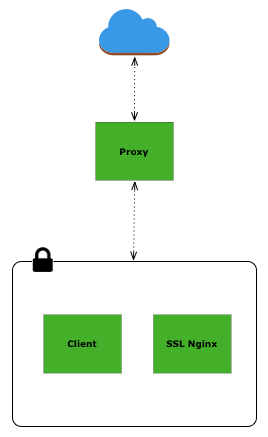
The default spill_device_limit is 80%. Let's lower it to 70%, and while we are at it, having easy access to the dashboard remotely would be quite helpful:

opts = StreamingOptions(
    spill_device_limit="70%",
)

ray_init_options = {
    "include_dashboard": True,
    "dashboard_host": "0.0.0.0",
    "dashboard_port": 8265,
}


with RayEngine.from_options(opts, ray_init_options=ray_init_options) as engine:
    query.sink_parquet(OUTPUT_DIR, engine=engine)

This time the query runs cleanly. In the GIF below, all four T4s turn on and stay busy for most of the query. That is the main thing I wanted to see. Our cycle has been: 1. Take a Polars query and naively run it on multiple GPUs. 1. Hit an OOM. 1. Tune the engine and re-run. 1. Success!

Speed anomaly query

I'm not terribly confident in the domain analysis. On the surface it seems plausible, but it probably deserves more scrutiny from someone who knows AIS data better than I do. As a systems exercise, though, this is exactly the kind of workload I hoped for: large enough to require multi-GPU execution, memory intensive enough to require spilling, and communication-heavy enough to make the execution engine do real distributed work.

In [10]: (
    ...:       pl.scan_parquet('/localhome/local-bzaitlen/ais-cudf-polars/output/result/*.parquet')
    ...:       .group_by('VesselType')
    ...:       .agg(pl.len().alias('anomaly_count'))
    ...:       .sort('anomaly_count', descending=True)
    ...:       .limit(5)
    ...:       .collect()
    ...:       .with_columns(
    ...:           pl.col('VesselType').map_elements(lambda x: VESSEL_TYPES.get(x, f"Unknown ({x})"), retur
       ⋮ n_dtype=pl.String).alias('VesselTypeName')
    ...:       )
    ...:   )
Out[10]:
shape: (5, 3)
┌────────────┬───────────────┬───────────────────┐
│ VesselType ┆ anomaly_count ┆ VesselTypeName    │
│ ---        ┆ ---           ┆ ---               │
│ i64        ┆ u32           ┆ str               │
╞════════════╪═══════════════╪═══════════════════╡
│ 52         ┆ 547390        ┆ Tug               │
│ 30         ┆ 262985        ┆ Fishing           │
│ 70         ┆ 252750        ┆ Cargo             │
│ 60         ┆ 216759        ┆ Passenger         │
│ 51         ┆ 193884        ┆ Search and rescue │
└────────────┴───────────────┴───────────────────┘

Turns out it's mostly the Tugs which operate at 10x the average speed. I suppose that makes some sense; Little Toot liked the figure-eights in the harbor but could only go so fast when pulling in the big ocean liners.

Fancy Memory for ETL pt. 2

Pinned memory changes both the cost of each transfer and the behavior of the pipeline. It pays an upfront allocation cost, but can reduce spill overhead, lower memory pressure, and improve end-to-end runtime

In the previous post, I explored how spilling can enable larger-than-VRAM workloads to run on a GPU. Spilling comes with a cost, but pinned memory can reduce memory transfer bottlenecks. In this post, I want to dive a little deeper into what's happening with pinned and pageable memory. To do that exploration, we'll use Nsight Systems (nsys) which can give us detailed profiling information on the workflow I developed in pt 1.

nsys profile -o pageable-spill -f true -t cuda,nvtx --stats=false python script.py

Full Timeline View

As a reminder, I measured the same join workflow which requires more VRAM than an L40 has (48GB) using two different memory types: regular/pageable host memory: 27s and pinned host memory: 23s. Those numbers are the query execution times after engine initialization. The pinned-memory Nsight trace below also includes the one-time pinned-memory pool initialization and explains why we see more than 23s of time in the trace.

Trace with pageable (non-pinned) memory 
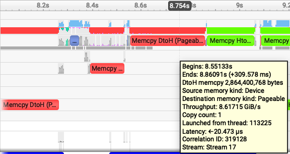
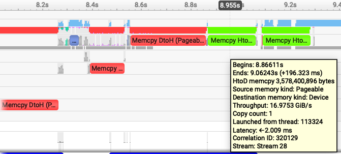
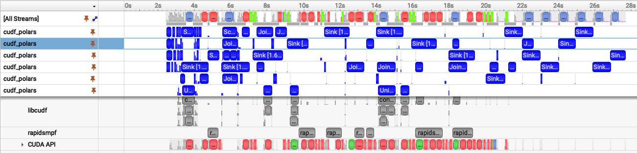
Fig 1. Nsight Systems timeline showing the pageable-memory cudf-polars join workflow.

Trace with pinned memory 
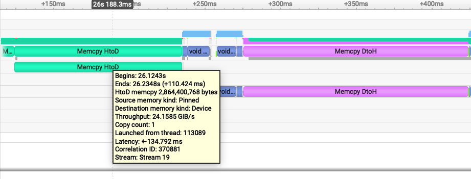
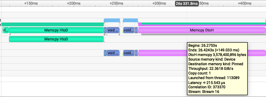
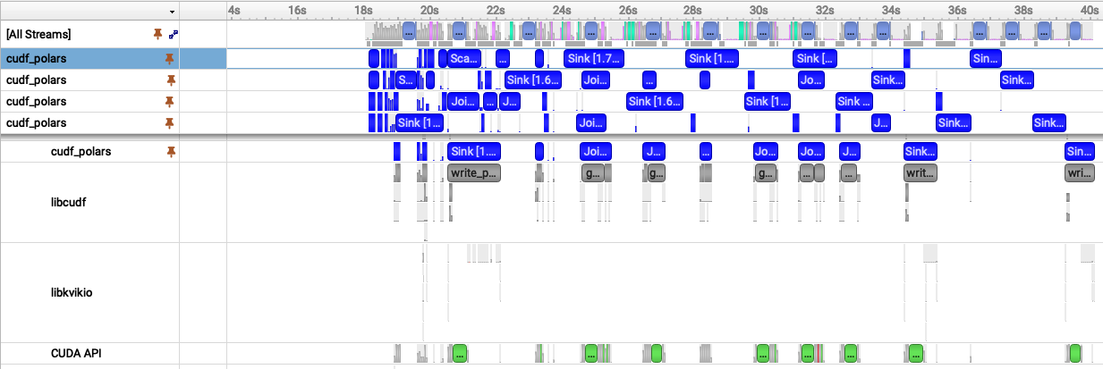
Fig 2. Nsight Systems timeline showing the pinned-memory cudf-polars join workflow.

With these two images laid out together, we can visually see similarities and differences:

  1. Both have multiple cudf_polars streams (blue bars) though Fig 1. has 6 and Fig 2. has 5 -- let's come back to that
  2. With pageable memory (fig 1) we see a load of red and green transfer bars and they start near the 2s mark
  3. With pinned memory (Fig. 2), the transfer bars are narrower than the pageable transfer bars in Fig. 1, meaning each transfer takes less time. The query work also starts near the 18s mark because the first ~18s are spent allocating the pinned memory pool.

As a reminder, here's the aggregate time spent spilling (device-to-host) and unspilling (host-to-device) for both memory types:

Mode Direction Time
Pageable host spilling Device -> host 8.06 s
Pageable host spilling Host -> device 4.06 s
Pinned host spilling Device -> pinned host 2.64 s
Pinned host spilling Pinned host -> device 3.15 s

It's interesting: pageable host spilling is slower when moving data Device->Host compared with Host->Device. However, when using pinned memory, the throughput in both directions is nearly the same. Why? Zooming into a region where the workflow is spilling can help us see why.

Zooming In: Pageable Memory

Pageable device -> host Pageable host -> device
Pageable device to host transfer detail Pageable host to device transfer detail

nsys lets us easily see not just how much time was spent spilling, but also how much data was transferred, and data/time gives us a throughput measurement. The following images are samples, each transfer will have some noise (a few may have spikes), but these are representative. In the zoomed-in images, Device->Host is 8.6GiB/s and Host->Device is ~17 GiB/s. When transferring data using regular pageable memory, the host has to first allocate memory before the device can spill and it's apparently quite costly to do this. When moving data back to the device, there is no allocation cost so it's significantly faster.

Quick aside: cuDF-Polars and RapidsMPF use CUDA’s stream-ordered allocator, cudaMallocAsync, by default. It’s fairly technical, but the short version is that cudaMallocAsync avoids many costly device-wide synchronization points by making allocation and free operations stream-ordered.

Zooming In: Pinned Memory

Let's do the same kind of inspection of the pinned memory nsys plot:

Pinned host -> device Pinned device -> host
Pinned host to device transfer detail Pinned device to host transfer detail

Device->Host data movement is a lot faster: 24 GiB/s and Host->Device is 22GiB/s. Pinned memory throughput is so much faster because we paid all the host memory allocation fees during initialization. The host doesn't have to allocate any memory -- it's already there for the device to use!

Why though is Host->Device faster for pinned memory compared with pageable memory? It's great fun getting an excuse to learn about how machines actually work. We aren't going to dive very deep, but just peer into the depths without falling too far in.

When the host allocates pageable memory, the operating system is still largely in control of that memory and still responsible for running the entire machine! The OS can move the memory to another physical location or even swap it to disk. This means the host, the OS, is responsible for moving the data and safeguarding the memory from corruption during the process. It’s safe but slow, and one of the primary reasons why Direct Memory Access (DMA) was created to let devices transfer data directly to and from memory, reducing CPU involvement in the copy path. In a way, it’s one of the freedoms, or footguns, the OS gives back to the application developer.

Interestingly, DMA dates back to computing in the 50s, when many of these ideas around pipelining and overlapping execution were already taking shape.

So, Host->Device is faster with pinned memory because the host memory is pagelocked. Since those pages cannot be moved or swapped out by the OS during the transfer, the GPU can use DMA to copy directly from host memory to device memory, avoiding the extra staging and CPU/OS overhead required for pageable memory.

With nsys we can start to see why pinned memory and DMA can be so impactful. (We may explore RDMA/GPUDirect RDMA in a later post.)

Why Copy Time Is Not Wall-Clock Time

So far we have looked at individual transfer costs; now let's connect that back to the full query timeline. Why, if we spend 12 seconds spilling with pageable memory and only 5 seconds spilling with pinned memory, do we not see wall-clock time reduced by 7 seconds?

It's understandably confusing because cuDF-Polars and RapidsMPF are doing work concurrently and, when the hardware allows it, in parallel. Spilling is not a single serial phase that blocks the whole query. This is pipelining; different chunks of the query can be in different stages at the same time. One chunk may be spilling to host, another may be unspilling back to the device, and another may be running libcudf kernels.

CUDA work in a single stream is ordered, Kernel A -> allocate memory -> Kernel B -> free memory happens sequentially. But work submitted to different streams can overlap. RapidsMPF manages the pipeline for us, which is why the spill times do not translate directly into overall execution time.

This is also a good time to return to the stream-count puzzle from the nsys profiles at the beginning.

Both have multiple cudf_polars streams (blue bars) though Fig 1. has 6 and Fig 2. has 5 -- let's come back to that

The pageable run shows six active cudf_polars streams, while the pinned run shows five. That does not mean pageable memory has better parallelism. We want higher perf and higher throughput, not necessarily more parallelism or more concurrency, though those traits often correspond to overall lower execution time. The pageable transfers are slower, so more chunks pile up in flight and nsys shows more active streams. Pinned memory moves data faster, reduces memory pressure faster, and lets the pipeline drain sooner.

With num_py_executors, cuDF-Polars sets the maximum number of Python worker threads available to drive RapidsMPF work. The number of active CUDA streams RapidsMPF uses depends on how much work the query exposes at runtime, plus memory pressure, dependencies, hardware availability, and backpressure building up in the pipeline.

Summary

Pageable spilling spends more time moving data and can make the trace look busier because work backs up. Pinned spilling pays an upfront allocation cost, but spends less time spilling during the query. For larger out-of-core workflows, that can mean better throughput, less memory pressure, and fewer OOM surprises.

Fancy Memory for ETL pt. 1

Spilling makes larger-than-VRAM GPU analytics possible, but memory movement is not free. For longer-running workflows or repeated queries, using pinned host memory can materially reduce memory movement overhead and decrease overall execution time.

My team recently released cuDF-Polars 26.06 which brings significant performance improvements over the previous versions, leveraging a new execution backend: RapidsMPF. Over the coming weeks and months I want to spend time highlighting some of the more advanced features and get into general ideas of how to build accelerated ETL engines.

Let’s start with a longstanding challenge for GPU analytics: running beyond available GPU memory. In the following example, we generate data larger than the GPU memory available and force the engine into a spilling path. Spilling means moving data from device memory to host memory when the operations would otherwise exceed available VRAM and cause an OOM.

Setting Up A Larger-Than-VRAM Query

For this example I found some time on an L40 GPU which you can easily rent on aws or any other major CSP. An L40 has 48 GB of GPU memory (VRAM), and this machine also comes with a considerable amount of CPU resources: 128 GB of RAM and an AMD EPYC 7313P 16-Core Processor.

Let's first start by generating some data. I had an agent build me some wholesale order like data with tables: lineitem, orders, customers, and suppliers.

Data Generation Code

Rows: lineitem=95,000,000, orders=23,750,000, customer=2,375,000, supplier=200,000
Generated 3.74 GiB compressed on disk
Data generation took 39.80 seconds

As an aside, using AI agents to quickly generate data is handy. For synthetic examples like this where I'm more interested in showcasing a feature than a specific use case, it’s just a faster way to get to the actual code and start benchmarking.

Great! We've got some data, how about a query? Let's go after a more complex query, not too long -- something with joins and some zest -- large enough to stress memory:

Full working example

def build_query(data_dir: Path = DATA_DIR) -> pl.LazyFrame:
    lineitem = pl.scan_parquet(str(data_dir / "lineitem-*.parquet"))
    orders = pl.scan_parquet(str(data_dir / "orders-*.parquet"))
    customer = pl.scan_parquet(str(data_dir / "customer-*.parquet"))
    supplier = pl.scan_parquet(str(data_dir / "supplier-*.parquet"))

    return (
        lineitem.join(orders, on="orderkey", how="inner")
        .join(customer, on="custkey", how="inner")
        .join(supplier, on="suppkey", how="inner")
        .with_columns(
            [
                (pl.col("extendedprice") * (1.0 - pl.col("discount"))).alias(
                    "net_revenue"
                ),
                (pl.col("quantity") * pl.col("supply_cost")).alias("supply_value"),
                (pl.col("ship_day") - pl.col("order_day")).alias("ship_lag_days"),
            ]
        )
    )

Uncompressed the data is ~50GB, so we'd expect some spilling. With cuDF-Polars 26.06, we have a new backend to execute and manage memory: RapidsMPF. Let's see what happens when we naively run the query and write the results back to disk:

build_query(data_dir).sink_parquet(output_path, engine='gpu')

Spilling Saves The Query

On this L40, the query runs in ~27s. By default, at 80% of the device memory, cuDF-Polars will start spilling from device-to-host. Let's turn off spilling and see what happens. For this we are going to explicitly configure the GPU engine and options for cuDF-Polars:

options = StreamingOptions(
    spill_device_limit="100%"
)
engine = SPMDEngine.from_options(options)

build_query(data_dir).sink_parquet(output_path, engine=engine)

Running this we get an error!

MemoryError: Try lowering target_partition_size (current 1207644979) and/or RAPIDSMPF_SPILL_DEVICE_LIMIT (default '80%') to reduce peak memory. See https://docs.rapids.ai/api/cudf/stable/cudf_polars/memory_errors/ for troubleshooting guidance. Original error: std::bad_alloc: out_of_memory: CUDA error (failed to allocate 576000000 bytes) at: /tmp/conda-bld-output/bld/rattler-build_librmm/work/cpp/include/rmm/mr/cuda_async_view_memory_resource.hpp:87: cudaErrorMemoryAlloc

The default spill device limit of 80% feels like a good balance between performance and usability. It gives users a working out-of-core GPU analytics experience without requiring them to understand memory tuning up front. Now let’s keep the default spill limit (80%), enable statistics, and inspect what actually happened during execution.

options = StreamingOptions(
    statistics=True,
    fallback_mode="raise",
    spill_device_limit=SPILL_DEVICE_LIMIT,
)
engine = SPMDEngine.from_options(options)

build_query(data_dir).sink_parquet(output_path, engine=engine)

After running, calling engine.global_statistics(clear=True).to_dict() gives us a dictionary of stats collected by cudf-polars and RapidsMPF. The spill-related counters are the interesting ones for us in this experiment:

Mode Direction Bytes counter Count Total bytes Max transfer Time
Pageable host spilling Device -> host copy-device-to-host-bytes 24 70.34 GB 3.58 GB 8.06 s
Pageable host spilling Host -> device copy-host-to-device-bytes 24 70.34 GB 3.58 GB 4.06 s

Of the ~27s of execution, the workflow spends ~12s just copying spilled data between host and device. It moves about 70GB in each direction, so roughly 140GB crosses the PCIe boundary. That movement is expensive because of transfer bandwidth, allocating pageable memory on the host, and device synchronization points that can briefly pause streaming execution.

Pinned Memory Cuts The Copy Cost

If we use pinned memory and optimize data transfer between device and host we can speed up our execution BUT it comes with an initialization charge. It does take time for the OS to pre-allocate this memory upfront:

options = StreamingOptions(
    statistics=True,
    fallback_mode="raise",
    pinned_memory=True,
    pinned_initial_pool_size=100 * 1024**3,
    spill_device_limit="80%",
)

Engine initialization took ~16 seconds, but total execution time is now ~23s. For repeated or larger workloads, that upfront cost gets amortized: the engine pays the allocation cost once, then reuses the same pinned memory resource as more data moves through the pipeline. The spill volume is about the same, but the transfer portion is much faster in both directions.

Mode Direction Bytes counter Count Total bytes Max transfer Time
Pinned host spilling Device -> pinned host copy-device-to-pinned_host-bytes 23 67.47 GB 3.58 GB 2.64 s
Pinned host spilling Pinned host -> device copy-pinned_host-to-device-bytes 23 67.47 GB 3.58 GB 3.15 s
Mode Bytes copied each direction Total copy time Notes
Pageable host spilling 70.34 GB 12.11 s Regular host spilling copies through pageable host memory.
Pinned host spilling 67.47 GB 5.79 s Pinned transfers reduced copy time by 52.2%.

Spilling is a necessary component of accelerated analytics engines, especially on GPUs where memory is more constrained than system RAM. Pinned memory changes the cost of spilling by making the transfers much faster.

I expect this feature to become more widely used, but users should be aware of the one-time initialization cost. Making this policy opt-in keeps the tradeoff clear: startup may be slower, but larger or repeated workloads can achieve better performance with a simple configuration change.

While the stats tell us pinned memory substantially reduces transfer time, they do not show how that work overlaps with the rest of the query. In part 2, we’ll open Nsight Systems traces and look at what the pipeline is actually doing.

Integration Testing for the Enterprise

Written by Benjamin Zaitlen on 2016-11-21.

Building software for enterprises does not just mean more error checking (though it definitely does include that!), it means understanding a bit more about operations and IT. Each enterprise/organization has their own idea on how networking, security, authentication, and authorization are implemented; the variety can throw a big wrench in the reasonable assumptions often made in software tools deployed in those environments. It can be challenging to generalize these environments even with experiential knowledge (painful scars) and they can be even more challenging to test.

In this post, I want to tell you about a testing harness I made specifically for testing operational environments more commonly deployed by enterprise customers. As a motivating example I am going to test and validate that the package manager conda can correctly use proxies and self-signed certs.

The Problem

Proxies

If your tool/service needs to talk to the internet or generally be accessible throughout an organization it may need to use a proxy server. Proxies often act as intermediaries between a local intra-net and the global inter-net. (Late at night I think of proxies as mild-mannered pixies working at the Ministry of Regulated Communication.) In any case, many enterprise and corporate environments use proxies and thus your application will need proxy configurations possible.

Certs

Your tool may also need to download things occasionally, and that usually means handling SSL certificates. SSL certificates are primarily used to encrypt web traffic -- typically you see them in the URL name prefixed by HTTPS. In a follow up post I'll talk more about SSL certificate generation. Enterprises and their corporate intra-net, like the web at large, want to encrypt communication across the various services and tools which operate within it. Again, that means your tool needs to understand common SSL operations.

Solution

The good thing, of course, is that we don't have to build this all from the ground up -- someone else has already implemented all the technical bits, and your tools simply need to be configured appropriately.

In the case of conda, for example, handling proxies can be done in one of two ways: through a setting in the configuration file or with the common proxy environment variables https_proxy=proxy_url:port and https_proxy=proxy_url:port for the proxying of encrypted and unencrypted respectively. Conda knows how to handle proxies because Conda uses requests which knows how to properly handle proxies.

Similarly, Conda can use and validate encrypted communication with SSL certs with a configuration setting; it passes that info down to requests, and again, requests knows how to ssl verification

And if we dig deeper, requests can do it because urllib3 implemented SSL verification which in turn is dependent on pyopenssl. But now we are out of scope. The point here is that your new tool probably doesn't need to worry about all this because someone else did 99% of the work. What your tool needs to do is be configurable for these different communication patterns -- and that brings us to the test.

Testing!

We want to test the following: - conda install pkg behind a proxy - conda install pkg with a custom ssl cert

Network Image

The network above is a good illustration of a proxied network. We could build this network on AWS or any other cloud provider. I've found this fairly time consuming -- I'm not un-experienced when it comes to AWS, but I have trouble keeps VPC settings in my head and I will invariably mess up the the port routing in the security groups. Still, it's an option, though you do have the added burden of managing more machines and of course paying for the use.

Instead, we could reproduce this network not with cloud based machines but with Docker based containers. This has the advantage of not having to keep track of more AWS instances and its free of cost. Using docker also has the added benefit of being easily integrated into continuous integration tools like TravisCI

Proxy Testing

Since Docker 1.9, users have been able to define custom networks for the containers to exist in. What this means is that we can build containers in a network which is unable to communicate with the outside world. Below is an example of creating an isolated network named inside:

docker network create inside --internal --driver=bridge \
                   --subnet=192.168.99.0/24 --gateway=192.168.99.1 \
                   --ip-range=192.168.99.128/25

The key flag here is --internal and it disables communication between the containers and Docker's bridge to the host. Another interesting bit to note about Docker is that existing containers can be connected/disconnected from existing networks. So we can build three containers -- proxy, client, and ssl nginx -- and connect them all to the inside network; then connect the proxy to Docker's bridge network. The proxy container will then have access to the inside network and containers ssl nginx and client, as well as the outside -- hey that's exactly what a proxy does!

In the proxy container we use the tinyproxy proxy and prepopulate the config to allow the other containers. For our proxy test with conda we defined the environment variables https_proxy and http_proxy to install new conda packages

SSL Testing

Testing SSL verification with conda takes a bit more setup. We are going to need a DNS name, a webserver, some conda packages, and of course a valid cert. Luckily, Jamie Nguyen has a great guide on issuing custom certificates and I essentially used his method to build a cert for the DNS name proxy.io. To fake the DNS lookup I modified the /etc/hosts file with the IP of the SSL Nginx container. Great, so we have a valid dns name, a valid certificate for that name, we have the conda packages downloaded using the proxy method, and now we just need to serve them up.

To serve conda packages, we index them and start a server with python. Then we use nginx as a reverse proxy to that simple server and redirect all communication to https: nginx conf file

With a proper condarc file the client container can now install conda packages served over SSL on the SSL nginx container.

Conclusion

Testing software for enterprise configurations is possible and painful. It's painful because of the variety. I've found that Docker helps to mitigate that pain -- it's is flexible enough to handle the variety and easily integrates into larger testing harnesses. As proof, the full setup of the conda example describe above is hosted on github complete with continuous integration with TravisCI

SciPy Tutorial Setup On Kubernetes

Written by Benjamin Zaitlen on 2016-09-30.

This past summer I had the opportunity to work with Min Ragan-Kelley and Matthew Rocklin on delivering a tutorial at the scientific computing conference, SciPy 2016, in Austin, Texas. We set out to teach folks generally about parallel computing in the context of data analysis and not necessarily about any one tool. That is, focusing on core concepts rather than a specific framework. There is something strangely visceral when you are first learning about distributed computation and different hostnames pop up when executing a simple map across the cluster; and to that end, we wanted to give students access to a cluster capable of doing significant work -- something more than a toy. The tutorial was well received and all the content is publicly available:

Note: these materials will also be reused in an upcoming PyData Tutorial in Washington, DC

Many tutorials can get stuck (and sometimes fail) on setup and in the post I want to describe, in detail, our solution. We drew on our previous experiences running tutorials/trainings/lectures/etc. Our goal was to give students access to a preconfigured cluster with zero entry requirements: push a button get a cluster with all tools installed.

History

In graduate school, I helped with summer workshops teaching students, postdocs, and professors about Python in the context of biophysics and complex systems. Attendees showed up with a variety of machines and OSes: Linux, Windows, and OSX (both Intel and PPC). At least a collective day was spent getting our software and materials installed on all the machines so students could get hands on experience. Often our issues were handling multiple versions of Python but also odd bugs which invariably arise during trainings: permission errors, hard drive size limits, VPN blocking...

More recently, I helped build and run a tutorial at SciPy 2013: Data Processing with Python. Each student was given access to an individual clusters preconfigured with: Hadoop MapReduce, Disco, and IPython Parallel. It was a tremendous effort to stand this up and involved piles of bash, Python, and the magic of StarCluster -- and it all had to be setup before the class started with the caveat that total provisioning took ~5 hours. Still, it worked -- though, I was exhausted.

Hello Kubernetes

Not wanting to repeat the mistakes of the past and hearing great things about GCE and Kubernetes we committed early on to the Google Cloud Platform. Generously, Google donated resources for us to build out and iterate on our tutorial cluster platform. We are extremely appreciative of their support!

"Kubernetes is an open-source system for automating deployment, scaling, and management of containerized applications." What this means, is that if you have a service wrapped up in docker image, Kubernetes can help you do a number of things: deploy the image to a machine, scale the services and load balance between N containers, and handle things like auto-restarting, rolling upgrades, and generally the management that is often involved with running larger scale web services. Additionally, the Kubernetes cluster itself is fungible -- with a few button clicks, GKE can manage Kubernetes installed on a single medium-sized instance to dozens of extremely large instances. This is especially helpful when needing to scale computing resources as demand increases.

It's worth repeating that using Kubernetes does mean buying into the container ecosystem -- in our case that means Docker.

The Sea of Containers

An image

credit: http://panalpina.com/www/global/en/home/newsroom.html#/news/a-sea-of-containers-148839

Our goal was to give students access to a preconfigured cluster with zero entry requirements: push a button get a cluster with all tools installed. To accomplish this we need a handful of docker images:

  • Web application: button and info
  • Jupyter notebook
  • proxy app (more on this later)
  • cluster technologies: Spark, Dask, IPython Parallel

And a handful of Kubernetes concepts:

At a high level the web application launches a specific image within a unique namespace with requested resources, expose ports on the running containers, replicates some containers, and sets environment variables. And all of this, both the hardware resouces and the containers is being managed by Kubernetes. The web app is a Docker container, the proxy app is another Docker container, the namespaced clusters are a collection of Docker containers (the workers are replication controllers). It's Dockers as far as the eye can see!.

Architecture

I should also note that my friend and colleague, Daniel Rodriguez, contributed significantly to this effort and he worked out much of architecture and implementation with Kubernetes.

In building out this service we looked at previous work: mybinder and tmpnb. Both of these services launch temporary Jupyter notebooks using Docker. Similarly, we want a single page web application to launch a temporary Jupyter notebook connected to an isolated N-node cluster, where each cluster is running a variety of distributed computing engines -- also, we'd like to scale the number workers in the cluster.

An image

The button is pushed, a cluster+notebook is produced and the user is redirected to the running Jupyter notebook.

The Proxy

When we launch a container (Pod in Kubernetes) each Pod has an internal ip but it can optionally expose a publicly available ip and set of ports. If we want to support unique clusters for each button click, we either have to generate unique public IPs and hand them back to the user or proxy to the private IPs. Since we'd like to keep everyone on the same domain, we proxy to private IPs (see diagram above). Simply, this means that when a user goes to a running notebook at https://cluster.bigfatintegral.net/cluster-678343, for example, the proxy routes to the internal container. Below is an example of routing in the proxy:

"/cluster-678343":{"target":"http://10.20.1.17:8080","last_activity":"2016-08-23T19:51:43.091Z"},
"/cluster-678343_9000":{"target":"http://10.20.1.17:9000","last_activity":"2016-08-23T18:58:26.184Z"},
"/cluster-678343_9001":{"target":"http://10.20.1.17:9001","last_activity":"2016-08-23T19:03:14.741Z"},
"/cluster-678343_9002":{"target":"http://10.20.1.17:9002","last_activity":"2016-08-23T18:58:26.191Z"}

Note, that we proxy to four different PORTs with four URL endpoints:

  • /cluster-678343 -> 10.20.1.17:8080
  • /cluster-678343_9000 -> 10.20.1.17:9000
  • /cluster-678343_9001 -> 10.20.1.17:9001
  • /cluster-678343_9002 -> 10.20.1.17:9002

Where port 8080 routes to the Jupyter notebook, port 9000 routes to the Dask scheduler, and ports 9001 and 9002 route to the Dask's web interface. All the routes can be found here: http://173.255.119.91/api/routes.

Again, much of this architecture is heavily influenced by tmpnb and uses the same proxy app -- a small NodeJS app also built by the good folks from the Jupyter team: https://github.com/jupyterhub/configurable-http-proxy .

You may be wondering how the route was registered. Service discovery/auto-registration is a bit of magic and there are handful of tools to help with this problem. Consul/etcd/Zookeeper seem to be the popular choices -- however, in our case, we opted for something small and hand built; when a Pod is launched, the startup process includes a registration script which sends a POST containing the IP and the exposed PORT of the Pod to the proxy app. The proxy app holds the data in memory and waits for an incoming request to route to.

The App

The intro to Kubernetes has the user build out a small NodeJS Docker image and a YAML file. When used with the kubectl command, the YAML file instructs Kubernetes which kind of thing it is: a replicationController, a Service, a bare Pod, what ports to expose, etc. If you are familiar with docker-compose files many of the ideas map nicely. Instead of building these files and using the command line to build a cluster we want to use the Kubernetes API. Kubernetes does not provide a language based API. Instead, they provide a swagger spec and from this, swagger can generate valid Python (or any other language) objects and functions to properly interact with Kubernetes.

# how to generate a python swagger client
wget https://raw.githubusercontent.com/kubernetes/kubernetes/master/api/swagger-spec/v1.json
brew install swagger-codegen
swagger-codegen generate -i v1.json -l python

While this code generation is a good starting point, there are no docs provided to instruct you on how to use the API. Daniel is fantastic and started the process of trial and error, eventually building up an intuition for how to navigate the code. Below is an example of how we started to understand the namespace API. We want to use namespaces for each cluster launched because we want isolate virtual clusters.

We first noted two directories: swagger_client/models and swagger_client/apis. swagger_client/apis/apiv_api.py has many of the actions we want to perform with Kubernetes has and swagger_client/models has what looks like every model/spec for the Kubernetes universe of things. Let's look in swagger_client/models for something called namespace. Ah! v1_namespace.py seems like a good place to start. swagger_types looks like the spec in a YAML file: kind: Namespace. Look at the spec in the docs -- Ok, now we'll fail our way to success -- wait! How do we create namespace? Grep in swagger_client/apis/apiv_api.py for create and namespace and there are a bunch of functions. create_namespaced_namespace seems like a good place to start. The docstring says the body param is a V1Namespace object so let's start building an object

class NameSpace(V1Namespace):

    def __init__(self, name, proxy=None, *args, **kwargs):
        super(NameSpace, self).__init__(*args, **kwargs)
        self.kind = "Namespace"
        self.api_version = "v1"
        self.metadata.name = name

And we test:

ipdb> from .namespaces import NameSpace
ipdb> ns = NameSpace('hello')
ipdb> self.api.create_namespaced_namespace(ns)
*** core.swagger_client.rest.ApiException: (400)
Reason: Bad Request
HTTP response headers: HTTPHeaderDict({'Content-Length': '405', 'Date': 'Fri, 23 Sep 2016 17:30:04 GMT', 'Content-Type': 'application/json'})
HTTP response body: {"kind":"Status","apiVersion":"v1","metadata":{},"status":"Failure","message":"the object provided is unrecognized (must be of type Namespace): couldn't get version/kind; json parse error: json: cannot unmarshal string into Go value of type struct { APIVersion string \"json:\\\"apiVersion,omitempty\\\"\"; Kind string \"json:\\\"kind,omitempty\\\"\" } (2268656c6c6f22)","reason":"BadRequest","code":400}

It's not the most helpful of error messages -- but we keep hammering away at it until we've got the correct body contents. It goes like this until we get the NameSpace object correctly setup

With a functional API we can wrap various can now dynamically construct models and build namespaces as part of a web application. Using tornado seems like a good choice here since the app is mostly idling. Let's dig in a bit to what the cluster Docker setup is made of.

The Image

Not just any ordinary docker image, this image has it all!

  • Anaconda
  • Dask
  • Spark 2.0
  • IPython Parallel

This image is the core of the cluster; responsible for running all of the distributed computing engines and environment setup. When launched as a replication controller we can scale the workers to N containers. Notice that we only have one image -- we use the same image in two modes: scheduler and worker.

Note: normally the recommendation is to run one service per docker image -- in our case, we're going to run up to four. This is ok here mostly because the intended usage is to only work with one service at a time. The various schedulers and workers are idling and not consuming many resources (mem/cpu)

The modes of the same image are differentiated by the command executed when launching

The scheduler command registers the container with the proxy, starts a notebook server, and starts all the schedulers for Dask, Spark, and IPython Parallel. The worker command simply starts the workers for Dask, Spark, and IPython Parallel.

By declaring the workers as replicationControllers we can scale up and down the workers in a given cluster. This is done in a single tunable parameter. During the tutorial we also used the feature to show off the flexibility of Dask; with a running cluster executing a Dask job, we scaled the number of workers to 100 and Dask happily added 92 more workers to the job to the initial 8.

Outcomes

We ran the tutorial for a class size of 100+ students and additionally during Matt Rocklin's and Jim Crist's Dask Talk. I often worry and expect things to crash spectacularly and, in our case, everything went surprisingly well! The first part of the tutorial was designed to be executed on personal machines and, as I said mentioned before, personal machines come in all varieties of OSes and platforms -- and now, including tablets! We designed the cluster to clone all of our tutorial materials from Github so students, should install problems arise, could continue following along without a prolonged time resolving setup issues.

The cluster could run cheaply with a single medium sized instance and a few minutes before students arrived we provisioned additional resources. In total, each machine could have up to 2.0 vCPUs and 8GBs of RAM or a cluster with 16 vCPUs and 64 GBs of RAM.

Kubernetes more than lived up to the hype and again, we are very grateful to the generous support from Google in helping us build and share this with the PyData and SciPy communities.

Conda + Spark

Written by Benjamin Zaitlen on 2016-04-15.

In my previous post, I described different scenarios for bootstrapping Python on a multi-node cluster. I offered a general solution using Anaconda for cluster management and solution using a custom conda env deployed with Knit.

In a follow-up to that post, I was asked if the machinery in Knit would also work for Spark. Sure--of course! In fact, much of Knit's design comes from Spark's deploy codebase. Here I am going to demonstrate how we can ship a Python environment, complete with desired dependencies, as part of a Spark job without installing Python on every node.

Spark YARN Deploy

First I want to briefly describe key points in Spark's YARN deploy methodologies. After negotiating which resources to provision with YARN's Resource Manager, Spark asks for a directory to be constructed on HDFS: /user/ubuntu/.sparkStaging/application_1460665326796_0065/ The directory will always be in the user's home, and the application ID issued by YARN is appended to the directory name. (Thinking about this now, perhaps this is obvious and straightforward to JAVA/JVM folks where bundling Uber JARs has long been the practice in traditional Map-Reduce jobs.) In any case, Spark then uploads itself :) to the stagingDirectory, and when YARN provisions a container, the contents of the directory are pulled down and the spark-assembly jar is executed. If you are using PySpark or sparkR, a corresponding pyspark.zip and sparkr.zip will be found in the staging directory as well.

Occasionally, users see FileNotFoundException errors -- this can be caused by a few things: incorrect Spark Contexts, incorrect SPARK_HOME, and I have faint recollection that there was a packaging problem once where pyspark.zip or sparkr.zip was missing? or could not be created do to permissions? Anyway...below is the output you will see when Spark works cleanly.

16/04/15 13:01:03 INFO Client: Uploading resource file:/opt/anaconda/share/spark-1.6.0/lib/spark-assembly-1.6.0-hadoop2.6.0.jar -> hdfs://ip-172-31-50-60:9000/user/ubuntu/.sparkStaging/application_1460665326796_0065/spark-assembly-1.6.0-hadoop2.6.0.jar
16/04/15 13:01:07 INFO Client: Uploading resource file:/opt/anaconda/share/spark-1.6.0/python/lib/pyspark.zip -> hdfs://ip-172-31-50-60:9000/user/ubuntu/.sparkStaging/application_1460665326796_0065/pyspark.zip

Not terribly exciting, but positive confirmation that Spark is uploading local files to HDFS.

Bootstrap-Fu Redux

Mostly what I described above is what the YARN framework allows developers to do -- it's more that Spark implements a YARN application than Spark doing magical things (and Knit as well!). If I were using Scala/Java, I would package up everything in a jar and use spark-submit -- Done!

Unfortunately, there's a little more work to be done for an Uber Python jar equivalent.

One of the killer features of Conda is environment management. When Conda creates a new environment, it uses hard-links when possible. Generally, this greatly reduces disk usage. But, if we move the directory to another machine, we're probably just moving a handful of hard-links and not the files themselves. Fortunately, we can tell Conda: No! Copy the files!

For example:

conda create -p /home/ubuntu/dev --copy -y -q python=3 pandas scikit-learn

By using the --copy, we "Install all packages using copies instead of hard- or soft-linking." The headers in various files in the bin/ directory may have lines like #!/home/ubuntu/dev/bin/python. But we don't need to be concerned about that -- we're not going to be using 2to3, idle, pip, etc. If we zipped up the environment, we could move this onto another machine of a similar OS type, execute Python, and we'd be able to load any library in the lib/python3.45/site-packages directory.

We're very close to our Uber Python jar -- now with a zipped Conda directory in mind, let's proceed.

zip -r dev.zip dev

Death by ENV Vars

We are going to need a handful of specific command line options and environment variables: Spark Yarn Configuration and Spark Environment Variables. We'll be using:

  • PYSPARK_PYTHON: The Python binary Spark should use
  • spark.yarn.appMasterEnv.PYSPARK_PYTHON (though this one could be wrong/unnecessary/only used for --master yarn-cluster)
  • --archives: include local tgz/jar/zip in .sparkStaging directory and pull down into temporary YARN container

And we'll also need a test script. The following is a reasonable test to prove which Python Spark is using -- we're writing a no-op function which returns Python's various paths it is using to find libraries

# test_spark.py
import os
import sys
from pyspark import SparkContext
from pyspark import SparkConf

conf = SparkConf()
conf.setAppName("get-hosts")

sc = SparkContext(conf=conf)

def noop(x):
    import socket
    import sys
    return socket.gethostname() + ' '.join(sys.path) + ' '.join(os.environ)

rdd = sc.parallelize(range(1000), 100)
hosts = rdd.map(noop).distinct().collect()
print(hosts)

And executing everything together:

 PYSPARK_PYTHON=./ANACONDA/dev/bin/python spark-submit \
 --conf spark.yarn.appMasterEnv.PYSPARK_PYTHON=./ANACONDA/dev/bin/python \
 --master yarn-cluster \
 --archives /home/ubuntu/dev.zip#ANACONDA \
 /home/ubuntu/test_spark.py
 ```

 We'll get the following output in the yarn logs:
 >'ip-172-31-50-61 . /var/lib/hadoop-
yarn/data/1/yarn/local/usercache/ubuntu/filecache/207/spark-assembly-1.6.0-
hadoop2.6.0.jar /var/lib/hadoop-yarn/data/1/yarn/local/usercache/ubuntu/appcach
e/application_1460665326796_0070/container_1460665326796_0070_01_000003/{{PWD}}
/pyspark.zip<CPS>{{PWD}}/py4j-0.9-src.zip /var/lib/hadoop-yarn/data/1/yarn/loca
l/usercache/ubuntu/appcache/application_1460665326796_0070/container_1460665326
796_0070_01_000003/pyspark.zip /var/lib/hadoop-yarn/data/1/yarn/local/usercache
/ubuntu/appcache/application_1460665326796_0070/container_1460665326796_0070_01
_000003/py4j-0.9-src.zip /var/lib/hadoop-yarn/data/1/yarn/local/usercache/ubunt
u/appcache/application_1460665326796_0070/container_1460665326796_0070_01_00000
3/ANACONDA/dev/lib/python35.zip /var/lib/hadoop-yarn/data/1/yarn/local/usercach
e/ubuntu/appcache/application_1460665326796_0070/container_1460665326796_0070_0
1_000003/ANACONDA/dev/lib/python3.5 /var/lib/hadoop-yarn/data/1/yarn/local/user
cache/ubuntu/appcache/application_1460665326796_0070/container_1460665326796_00
70_01_000003/ANACONDA/dev/lib/python3.5/plat-linux /var/lib/hadoop-yarn/data/1/
yarn/local/usercache/ubuntu/appcache/application_1460665326796_0070/container_1
460665326796_0070_01_000003/ANACONDA/dev/lib/python3.5/lib-dynload
/var/lib/hadoop-yarn/data/1/yarn/local/usercache/ubuntu/filecache/208/dev.
zip/dev/lib/python3.5/site-packages/setuptools-20.6.7-py3.5.egg /var/lib/hadoop
-yarn/data/1/yarn/local/usercache/ubuntu/appcache/application_1460665326796_007
0/container_1460665326796_0070_01_000003/ANACONDA/dev/lib/python3.5/site-
packages ...',
'ip-172-31-50-62 . /var/lib/hadoop-
yarn/data/1/yarn/local/usercache/ubuntu/filecache/209/spark-assembly-1.6.0-
hadoop2.6.0.jar /var/lib/hadoop-yarn/data/1/yarn/local/usercache/ubuntu/appcach
e/application_1460665326796_0070/container_1460665326796_0070_01_000002/{{PWD}}
/pyspark.zip<CPS>{{PWD}}/py4j-0.9-src.zip /var/lib/hadoop-yarn/data/1/yarn/loca
l/usercache/ubuntu/appcache/application_1460665326796_0070/container_1460665326
796_0070_01_000002/pyspark.zip /var/lib/hadoop-yarn/data/1/yarn/local/usercache
/ubuntu/appcache/application_1460665326796_0070/container_1460665326796_0070_01
_000002/py4j-0.9-src.zip /var/lib/hadoop-yarn/data/1/yarn/local/usercache/ubunt
u/appcache/application_1460665326796_0070/container_1460665326796_0070_01_00000
2/ANACONDA/dev/lib/python35.zip /var/lib/hadoop-yarn/data/1/yarn/local/usercach
e/ubuntu/appcache/application_1460665326796_0070/container_1460665326796_0070_0
1_000002/ANACONDA/dev/lib/python3.5 /var/lib/hadoop-yarn/data/1/yarn/local/user
cache/ubuntu/appcache/application_1460665326796_0070/container_1460665326796_00
70_01_000002/ANACONDA/dev/lib/python3.5/plat-linux /var/lib/hadoop-yarn/data/1/
yarn/local/usercache/ubuntu/appcache/application_1460665326796_0070/container_1
460665326796_0070_01_000002/ANACONDA/dev/lib/python3.5/lib-dynload
/var/lib/hadoop-yarn/data/1/yarn/local/usercache/ubuntu/filecache/211/dev.
zip/dev/lib/python3.5/site-packages/setuptools-20.6.7-py3.5.egg /var/lib/hadoop
-yarn/data/1/yarn/local/usercache/ubuntu/appcache/application_1460665326796_007
0/container_1460665326796_0070_01_000002/ANACONDA/dev/lib/python3.5/site-
packages ...'


It's a little hard to parse -- what should be noted are file paths like:

> .../container_1460665326796_0070_01_000002/ANACONDA/dev/lib/python3.5/site-
packages

This is demonstrating that Spark is using the unzipped directory in the YARN container.  Ta-da!

## Thoughts

Okay, perhaps that's not super exciting, so let's zoom out again:

1. We create a zipped Conda environment with dependencies: pandas, python=3,...
2. We successfully launched a Python Spark job without any Python binaries or libraries
previously installed on the nodes.

There is an [open JIRA ticket](https://issues.apache.org/jira/browse/SPARK-13587) discussing
the option of having Spark ingest a `requirements.txt` and building the Python environment
as a preamble to a Spark job.  This is also a fairly novel approach to the same end -- using Spark
to bootstrap a runtime environment.  It's even
a bit more general, since the method described above relies on YARN. I first saw this strategy
in use with [streamparse](https://streamparse.readthedocs.org/).
Similarly to the implementation in JIRA ticket, [streamparse can ship a Python `requirements.txt`](https://streamparse.readthedocs.org/en/stable/quickstart.html#disabling-configuring-virtualenv-creation)
 and construct a Python environment as part of a Streamparse Storm job!

 ## Rrrrrrrrrrrrrr

 Oh, and R Conda environments work as well...but it's more involved:

 ### Create/Munge R Env

First, it's pretty cool that Conda can install and manage R environments.
Again, we create a Conda environment with R binaries and libraries

```bash
conda create -p /home/ubuntu/r_env --copy -y -q r-essentials -c r

R is not exactly relocatable so we need to munge a bit:

sed -i "s/home\/ubuntu/.r_env.zip/g" /home/ubuntu/r_env/bin/R
zip -r r_env.zip r_env

My R skills are at a below-novice level, so the following test script could probably be improved

# /home/ubuntu/test_spark.R
library(SparkR)
sc <- sparkR.init(appName="get-hosts-R")

noop <- function(x) {
  path <- toString(.libPaths())
  host <- toString(Sys.info()['nodename'])
  host_path <- toString(cbind(host,path))
  host_path
}


rdd <- SparkR:::parallelize(sc, 1:1000, 100)
hosts <- SparkR:::map(rdd, noop)
d_hosts <- SparkR:::distinct(hosts)
out <- SparkR:::collect(d_hosts)
print(out)

Execute (and the real death by options):

SPARKR_DRIVER_R=./r_env.zip/r_env/lib/R spark-submit --master yarn-cluster \
--conf spark.yarn.appMasterEnv.R_HOME=./r_env.zip/r_env/lib64/R \
--conf spark.yarn.appMasterEnv.RHOME=./r_env.zip/r_env \
--conf spark.yarn.appMasterEnv.R_SHARE_DIR=./r_env.zip/r_env/lib/R/share \
--conf spark.yarn.appMasterEnv.R_INCLUDE_DIR=./r_env.zip/r_env/lib/R/include \
--conf spark.executorEnv.R_HOME=./r_env.zip/r_env/lib64/R \
--conf spark.executorEnv.RHOME=./r_env.zip/r_env \
--conf spark.executorEnv.R_SHARE_DIR=./r_env.zip/r_env/lib/R/share \
--conf spark.executorEnv.R_INCLUDE_DIR=./r_env.zip/r_env/lib/R/include \
--conf  spark.r.command=./r_env.zip/r_env/bin/Rscript \
--archives r_env.zip \
/home/ubuntu/test_spark.R

Example output:

[[1]]
[1] "ip-172-31-50-59, /var/lib/hadoop-yarn/data/1/yarn/local/usercache/ubuntu/filecache/230/sparkr.zip, /var/lib/hadoop-yarn/data/1/yarn/local/usercache/ubuntu/filecache/229/r_env.zip/r_env/lib64/R/library"

[[2]]
[1] "ip-172-31-50-61, /var/lib/hadoop-yarn/data/1/yarn/local/usercache/ubuntu/filecache/183/sparkr.zip, /var/lib/hadoop-yarn/data/1/yarn/local/usercache/ubuntu/filecache/182/r_env.zip/r_env/lib64/R/library"

Dask + Yarn

Written by Benjamin Zaitlen on 2016-04-08.

In the past few months we've seen a number of posts about Dask. For those unfamiliar with it, Dask is an out-of-core parallel framework for data analysis. Some of the more recent examples (1, 2, 3) have demonstrated Dask's distributed capabilities -- leveraging not just multi-core architectures, but also multi-node clusters. We need a way to launch Dask workers on many machines in our cluster. In a small cluster we might do this by manually SSH-ing into many machines, using a job scheduler like SGE, or using the dec2 tool to provision and bootstrap on ec2. However, for larger clusters this approach breaks down, especially when the cluster is simultaneously running many parallel frameworks like Hadoop, Spark, Impala, etc. In this case we typically use a cluster resource manager like YARN to start and stop jobs on the cluster and to manage their execution environments. In this post, I demonstrate a toy example using the YARN resource manager.

Knit

Unfortunately for the Python community, YARN is a JVM based framework. Fortunately for the Python community, we (with special thanks to Niels Zeilemaker and support from Continuum Analytics) wrote Knit. Knit is a Python/Scala-based library which enables Python developers to request resources from YARN. As YARN is a container based resource manager, in addition to the job we wish to execute the job pack will also request container resources: number of containers, amount of memory, number of cores, queues, etc.

Dask+Knit

First, we start the scheduler on one of nodes -- typically, this will be an edge node or head node (a node where we can communicate with the YARN Resource Manager):

ubuntu@ip-172-31-62-166:~/$ dscheduler
distributed.scheduler - INFO - Start Scheduler at:        172.31.62.166:8786
distributed.scheduler - INFO -            http at:        172.31.62.166:9786

Dask is resilient to workers appearing and disappearing from the scheduler. With the scheduler up, we can add dworkers and point them at the scheduler's IP and port by issuing the following command:

$ dworker 172.31.62.166:8786

Using Knit, we'll use the same command above and start simply by asking for one container with YARN defaults for CPU and Memory:

>>> from knit import Knit
>>> k = Knit()
>>> cmd = "dworker 172.31.62.166:8786"
>>> appId = k.start(cmd, num_containers=1)
6/04/06 15:58:16 INFO knit.Client$: Staring Application Master
Attempting upload of /home/ubuntu/knit/knit/java_libs/knit-1.0-SNAPSHOT.jar
Uploading resource file:/home/ubuntu/knit/knit/java_libs/knit-1.0-SNAPSHOT.jar -> hdfs://ip-172-31-62-166.ec2.internal:8020/user/ubuntu/.knitDeps/knit-1.0-SNAPSHOT.jarhdfs://ip-172-31-62-166.ec2.internal:8020/user/ubuntu/.knitDeps/knit-1.0-SNAPSHOT.jar
16/04/06 15:58:20 INFO impl.TimelineClientImpl: Timeline service address: http://ip-172-31-62-167.ec2.internal:8188/ws/v1/timeline/
16/04/06 15:58:20 INFO client.RMProxy: Connecting to ResourceManager at ip-172-31-62-167.ec2.internal/172.31.62.167:8050
Security is enabled: true
16/04/06 15:58:20 INFO hdfs.DFSClient: Created HDFS_DELEGATION_TOKEN token 162 for ubuntu on 172.31.62.166:8020
[Lorg.apache.hadoop.security.token.Token;@5fdbded6
Got dt for DFS[DFSClient[clientName=DFSClient_NONMAPREDUCE_-453042160_12, ugi=ubuntu@CONTINUUM (auth:KERBEROS)]].getUri() Kind: HDFS_DELEGATION_TOKEN, Service: 172.31.62.166:8020, Ident: (HDFS_DELEGATION_TOKEN token 162 for ubuntu)
16/04/06 15:58:20 INFO knit.Client$: Submitting application application_1458491078518_0071
16/04/06 15:58:21 INFO impl.YarnClientImpl: Submitted application application_1458491078518_0071

The scheduler will verify that a new worker has connected:

distributed.core - INFO - Connection from 172.31.62.167:58512 to Scheduler
distributed.scheduler - INFO - Register 172.31.62.167:42748

Let's kill the YARN application and now ask for 5 containers:

>>> k.kill()
16/04/06 16:51:00 INFO impl.YarnClientImpl: Killed application application_1458491078518_0071

>>> appId = k.start(cmd, num_containers=5)

Again, the scheduler will also confirm we have new dworkers:

distributed.core - INFO - Connection from 172.31.62.167:39885 to Scheduler
distributed.scheduler - INFO - Register 172.31.62.167:43795
distributed.core - INFO - Connection from 172.31.62.169:60726 to Scheduler
distributed.scheduler - INFO - Register 172.31.62.169:52115
distributed.core - INFO - Connection from 172.31.62.166:33672 to Scheduler
distributed.scheduler - INFO - Register 172.31.62.166:37686
distributed.core - INFO - Connection from 172.31.62.169:60727 to Scheduler
distributed.scheduler - INFO - Register 172.31.62.169:51797
distributed.core - INFO - Connection from 172.31.62.166:33673 to Scheduler
distributed.scheduler - INFO - Register 172.31.62.166:33068

Five Dask workers are now running in various YARN containers throughout our cluster -- we can now connect an Executor to the scheduler and begin our analytics processing with Dask.

>>> from distributed import Executor
>>> e = Executor('172.31.62.166:8786')

....

Bootstrap-Fu

What wasn't mentioned in all of this is how we bootstrapped the cluster with Python, Dask, Knit, and all the other goodies. In this particular case, I used Anaconda for cluster management. This is an especially useful tool for both bootstrapping and managing Python (and R) remotely.

I would recommend folks check out Anaconda for cluster management -- but still, there are times when we don't need a hammer when a chisel will do. Within Knit, we have such a chisel. Knit can create a small but complete Python environment -- with the dependencies you need -- and ship this env along with your command. This is immeasurably valuable to those curious and excited about bringing the PyData stack to Hadoop. For example, let's build and ship an env with Dask, Pandas, and Scikit-Learn and assume we are starting on a blank cluster.

$ conda/pip install knit
$ python
>>> from knit import Knit
>>> k = Knit()
>>> env_zip = k.create_env(env_name='dev', packages=['python=3', 'distributed',
...                                                  'dask', 'pandas', 'scikit-learn'])


>>> cmd = '$PYTHON_BIN $CONDA_PREFIX/bin/dworker 172.31.62.166:8786'
>>> appId = k.start(cmd=cmd, env=env_zip)
...

And we're done! We've given the PyData community the space to leverage powerful tools we know and love in a previously non-friendly Python ecosystem.

Future Work

While we've demonstrated Dask on YARN, it's more cumbersome than I would like. It would be better if the Scheduler talked directly to YARN and we have an open issue discussing what that interface may look like. We are also pursuing other tasks, namely: