Out-Of-Core Shuffling w/ RapidsMPF

Shuffling data at 1.8 TiB/s! RapidsMPF is a reusable, out-of-core shuffler that turns shuffling OOM headaches into a spill you can budget for.

Shuffling is the crux of structured data analytics distributed or otherwise. It's a core component of key data operations like: join, groupby, merge, sort, etc. A full distributed shuffle can move all the data from every process to every other process, an all-to-all. This is very costly and many sophisticated techniques have been developed to avoid this operation as much as possible. Shuffles aren't particularly computationally challenging: calculating the hashes to route data is fairly cheap. They are nonetheless expensive in a workflow, for a variety of reasons:

Memory intensive: shuffles can require holding onto a full copy of all the data or, in streaming cases, memory pressure can build and cause OOMs.
Transport: The data physically has to be moved from Process A->Process B or Node A->Node B so it can only move at speed of the transport layer.
Synchronization: Output data cannot be consumed until all producers have finished contributing data. In a bulk-synchronous engine, this barrier can stall the entire execution plan.

Because shuffling is hard, slow, memory-intensive, and critical, it's historically where RapidsMPF started.

Why do Joins need Shuffles?¶

A quick primer on joining tables. If we have two tables: partsupp and lineitem and we want to join them, what happens?

partsupp.join(
   lineitem,
   left_on=["ps_partkey", "ps_suppkey"],
   right_on=["l_partkey", "l_suppkey"],
)

# or 

SELECT *
FROM partsupp
JOIN lineitem
  ON partsupp.ps_partkey = lineitem.l_partkey
 AND partsupp.ps_suppkey = lineitem.l_suppkey

In-Memory Joins¶

Inner joins are composed of two phases:

build phase: the smaller table (partsupp) is scanned and a hash table is constructed over the join keys (ps_partkey, ps_suppkey), mapping each hashed key to the row it came from. This hash table is fully populated before the probe phase can begin.
probe phase: the larger table (lineitem) is scanned and each row's keys (l_partkey, l_suppkey) are hashed. Matches between the hash of the build and probe table join keys emit an output row combining columns from both tables. Rows without matches are dropped (technically, there's also hash collision handling here, but ignore that for now).

note: left, right, and full outer joins use the same build/probe strategy with different rules for unmatched rows

At minimum, this in-memory join holds three tables: the build table, the probe table, and the output table and the hash table built over the build side.

Distributed Join¶

In the in-memory case, all the data is already colocated within the same memory space. That's no longer true once the tables are spread across many processes/nodes/ranks or tables are batched for "streaming" joins. A rank/process can only join rows in resident memory. Eventually, an in-memory join will occur, but first we'll need to get all the matching keys for the build and probe tables on the samerank.

The cartoon graphic below represents how various rows of the same color are shuffled into the same output partition, and those partitions live on different ranks.

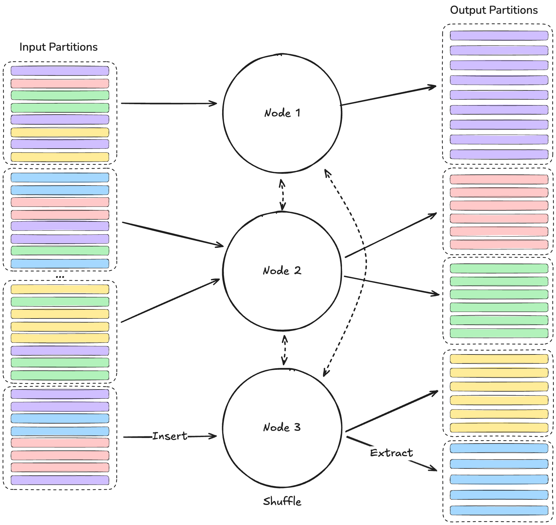
To execute a distributed hash-join one must do the following:

Scan the build table, hash the join keys of each row to pick a destination partition, hash(keys) % n_out_partitions. Pack and send each row to the rank that will own it.
Scan the probe table and route the rows the same way so that probe keys land on the rank already holding the build keys with the same hash.
Wait until every rank has finished sending. Only then is a rank guaranteed to hold every row, from both tables, for the keys it owns.
Run the in-memory join from above on each rank's local slice: build a hash table over its build rows, probe it with its probe rows, emit matches.

In the worst case, if every stage is fully materialized before the next one begins, a single rank is holding all of the following at once:

build table (source scan)
probe table (source scan)
staged build table (packed for send)
staged probe table (packed for send)
shuffled build slice (received)
shuffled probe slice (received)
hash table over the build slice
output table

This is why shuffling is memory intensive rather than compute intensive. The hashing itself is cheap and it's why an out-of-core shuffle implementation should be a primary focus when setting out to build an ETL engine. Additionally, being able to stream data rather than fully materialize the tables before shuffling is critical for reducing memory pressure. For these reasons, we started RapidsMPF with the original goal of building a streaming out-of-core shuffler.

RapidsMPF¶

RapidsMPF has expanded since its original conception. It is now a library composed of two large pieces: 1. A shuffle library designed for spilling / out-of-core memory handling, with accelerated transport 1. An actor network for constructing streaming data pipelines

Users today can still adopt just the shuffling component of RapidsMPF (C++ or Python interfaces). We've seen this adoption in NeMo-Curator and, experimentally, in Ray Data. Most importantly, cuDF Polars uses RapidsMPF for both shuffles and the actor network.

In a follow-up post we can dive into the actor network or if you're curious now I'd recommend reading the section on the streaming engine.

Our shuffle implementation needs to:

Be fast
Scale
Work with larger than VRAM (GPU) data (out-of-core)
Be reusable

and in the rest of this blog we'll focus our attention on shuffling under memory pressure.

Benchmarking Setup¶

cuDF/RapidsMPF has an easy-to-use C++ benchmark: bench_shuffle which helps us study how the RapidsMPF shuffling implementation works across varied hardware: transports, number of GPUs, etc, as well as varied configuration like: input/output partition sizes, memory resources, etc.

Here's a full breakdown of what the current bench_shuffle test exposes to users, along with the values I use throughout this post. Generally speaking, this benchmark builds tunable amounts of random 32-bit (4 byte) integers per rank (per GPU), shuffles all the data, and completes (there is no join here, just the shuffle).

Flag	Meaning	Values used here
`-C <name>`	Communicator	`ucxx`
`-c <n>`	Number of columns	`10`
`-r <n>`	Number of timed runs	`10`
`-w <n>`	Number of warmup runs	`3`
`-n <n>`	Number of rows per rank	`536870912` (2 GiB per column at 4 bytes/row)
`-p <n>`	Number of input partitions per rank	`1`
`-o <n>`	Number of output partitions per rank	`8` (one per rank)
`-m <name>`	RMM memory resource	`pool`
`-l <n>`	Device memory limit in MiB	omitted = unlimited (binary default `-1`); `32768` down to `12288` in the spill sweep
`-s`	Enable output discard (simulate streaming)	flag, always set
`-x`	Enable memory profiling	flag, always set
`-g`	Use pre-partitioned input tables	flag, always set

For all tests we are going to use a single DGXB200 and we are going to use rrun, an mpi like multiprocess launch tool capable of binding processes to NUMA nodes, to launch the shuffles.

Simple Shuffling¶

A DGXB200 has 8 Blackwell GPUs, each with 180GBs of VRAM, and 2 Intel® Xeon® Platinum 8570 Processors. To get a baseline, we'll start by shuffling data which comfortably fits across all GPUs.

rrun -n 8 --bind-to cpu --bind-to memory -x UCX_MAX_RNDV_RAILS=1 -x UCX_PROTO_ENABLE=y -x UCX_WARN_UNUSED_ENV_VARS=n libcudf_streaming_bench_shuffle -C ucxx -w 3 -r 10 -m pool -g -s -x -p 1 -o 8 -c 10 -n 536870912

Here we are warming up the benchmark 3 times, then running the benchmark 10 times. There are 536_870_912 rows (-n), 10 columns (-c), 1 input partition per rank (-p), and the data will be shuffled into 8 output partitions (-o). We are also using UCXX/UCX to enable accelerated transport/GPUDirect RDMA.

536_870_912 rows * 4 bytes (32-bit ints) = 2 GiB per column 10 columns * 2 GiB = 20 GiB / rank 8 ranks * 20 GiB = 160 GiB total

# example output for 20GiB/rank
[6:PRINT:0:2026-09-16 02:09:53.934930934] elapsed: 17.91 s | local throughput: 1.12 GiB/s | global throughput: 8.93 GiB/s (warmup run)
[5:PRINT:0:2026-09-16 02:09:53.935046244] elapsed: 17.91 s | local throughput: 1.12 GiB/s | global throughput: 8.93 GiB/s (warmup run)
[4:PRINT:0:2026-09-16 02:09:54.072443638] elapsed: 94.58 ms | local throughput: 211.47 GiB/s | global throughput: 1.65 TiB/s (warmup run)
[2:PRINT:0:2026-09-16 02:09:54.072450366] elapsed: 89.15 ms | local throughput: 224.35 GiB/s | global throughput: 1.75 TiB/s (warmup run)
[0:PRINT:0:2026-09-16 02:09:54.328272061] elapsed: 86.89 ms | local throughput: 230.19 GiB/s | global throughput: 1.80 TiB/s
[1:PRINT:0:2026-09-16 02:09:54.328286361] elapsed: 85.38 ms | local throughput: 234.25 GiB/s | global throughput: 1.83 TiB/s
[7:PRINT:0:2026-09-16 02:09:54.328417037] elapsed: 84.58 ms | local throughput: 236.47 GiB/s | global throughput: 1.85 TiB/s
[4:PRINT:0:2026-09-16 02:09:54.328429082] elapsed: 85.15 ms | local throughput: 234.87 GiB/s | global throughput: 1.83 TiB/s
[2:PRINT:0:2026-09-16 02:09:54.328554677] elapsed: 86.28 ms | local throughput: 231.80 GiB/s | global throughput: 1.81 TiB/s

Each rank posts how much time it spent shuffling, and the local and global throughput. Already we can observe that warming up has some cost as it runs slower than the "official" run. At the end, the program returns the average values per rank of local/global throughput and summary statistics per rank for where time was spent: time in shuffle, time allocating memory, spilling (if any), etc.

Note

The global throughput varies from rank to rank, which is technically wrong and is a reporting bug. Rather than summing the local throughputs across ranks, the benchmark reports the global throughput as each rank's own local throughput multiplied by the number of ranks. On a DGXB200 it's 8 x local throughput. But it will suffice for now while the bug is resolved.

[0:PRINT:0:2026-09-16 02:09:55.476576210] means: 87.06 ms | local throughput: 229.74 GiB/s | global throughput: 1.79 TiB/s | in_parts: 1 | out_parts: 8 | nranks: 8 | device memory peak: 60 GiB | device memory total

[0:PRINT:0:2026-09-16 02:09:55.476629379] Statistics (of the last run):
 - alloc-device:                                       17.50 GiB | 1.73 ms | 9.90 TiB/s | avg-stream-delay 213.98 us
 - event-loop-total:                                   3.44 ms | avg 2.29 us
 - metadata-payload-exchange-complete-data-transfers:  518.71 us | avg 345.80 ns
 - metadata-payload-exchange-progress:                 2.35 ms | avg 1.57 us
 - metadata-payload-exchange-receive-metadata:         558.98 us | avg 372.65 ns
 - metadata-payload-exchange-send-messages:            557.40 us
 - metadata-payload-exchange-setup-data-receives:      617.31 us | avg 411.54 ns
 - shuffle-payload-recv:                               17.50 GiB | avg 319.95 MiB
 - shuffle-payload-send:                               17.50 GiB | avg 320.01 MiB

Memory Profiling
----------------
Legends:
  ncalls - number of times the scope was executed.
  peak   - peak memory usage by the scope.
  g-peak - global peak memory usage during the scope's execution.
  accum  - total accumulated memory allocations by the scope.
  max    - largest single allocation by the scope.

Ordered by: peak (descending)

  ncalls        peak      g-peak       accum         max  filename:lineno(name)
       1      60 GiB      60 GiB    1.29 TiB       2 GiB  main (all allocations using RmmResourceAdaptor)
       1      40 GiB      40 GiB   44.06 GiB       2 GiB  /libcudf_streaming/src/partition_utils.cpp:183(partition_and_pack)
       1      20 GiB      20 GiB      20 GiB  320.39 MiB  /libcudf_streaming/src/partition_utils.cpp:242(split_and_pack)
       8    2.50 GiB    2.50 GiB      20 GiB  256.12 MiB  /libcudf_streaming/src/partition_utils.cpp:298(unpack_and_concat)
       1         0 B         0 B         0 B         0 B  /libcudf_streaming/benchmarks/bench_shuffle.cpp:277(shuffling)
       4       5 GiB       5 GiB      20 GiB  512.17 MiB  /libcudf_streaming/src/partition_utils.cpp:136(unpack_and_concat)
       1         0 B         0 B         0 B         0 B  /libcudf_streaming/benchmarks/bench_shuffle.cpp:276(shuffling)

In the above only rank 0 is provided, however, ranks 1-7 are very similar. Ranks do finish at slightly different times and will also have small but measurable variations in throughput. Given we have 1,440 GB VRAM across the eight GPUs, RapidsMPF has plenty of room to shuffle without needing to spill. In the above configuration, RapidsMPF drives roughly 1.8 TiB/s of global throughput. We still aren't at the theoretical ceiling of 14.4 TB/s but that's very fast!

The memory profile is worth a deeper look, because it will help us reason about spilling later on. Each rank only holds 20 GiB of input, but the peak device usage is 60 GiB, 3x the input. The profile shows exactly where it goes, 20 GiB for the input itself and 40 GiB in partition_and_pack while the input is hashed and copied into per-destination buffers. In a shuffle, the program may transiently own both the original and the copy of the local data; a good motivation for why we need to think deeply about memory management in all stages of the pipeline.

When shuffles are a required piece of the workflow, data comes in a variety of different partition sizes, shapes, and types, and GPUs vary in the amount of VRAM. We therefore should expect throughput to change as the shape and size of the data as well as the workflow overall changes. For now, we'll continue using the same setup of single 20GiB input partitions.

Oops, you spilled a little...¶

Each rank will initialize with 20 GiB of data and then shuffle. However, we are going to continually increase the memory pressure by lowering the device limit from no limit to 12GiBs. What we are going to observe is that not only does it not OOM, RapidsMPF doesn't thrash with unnecessary data movement back and forth between device and host. Note, we aren't putting this particular system at risk of OOMing. Instead, we are limiting the setup to 20 GiB of data/rank because we want to quickly simulate and interrogate what happens when the system is at risk of OOM-ing.

Let's apply some artifical memory pressure to the benchmark and limit the device to 32GB: -l 32768 and see what happens:

[7:PRINT:0:2026-09-16 02:10:59.613588706] means: 335.15 ms | local throughput: 59.67 GiB/s | global throughput: 477.39 GiB/s | in_parts: 1 | out_parts: 8 | nranks: 8 | device memory peak: 60 GiB | device memory tot
al: 101.56 GiB (avg)

[7:PRINT:0:2026-09-16 02:10:59.613648285] Statistics (of the last run):
 - alloc-device:                                       17.50 GiB | 8.11 ms | 2.11 TiB/s | avg-stream-delay 598.60 us
 - alloc-pinned_host:                                  5.62 GiB | 844 us | 6.51 TiB/s | avg-stream-delay 170.46 us
 - copy-pinned_host-to-device:                         5.62 GiB | 171.80 ms | 32.74 GiB/s | avg-stream-delay 1.78 ms
 - event-loop-total:                                   11.88 ms | avg 1.99 us
 - metadata-payload-exchange-complete-data-transfers:  1.09 ms | avg 183.69 ns
 - metadata-payload-exchange-progress:                 9.76 ms | avg 1.64 us
 - metadata-payload-exchange-receive-metadata:         1.24 ms | avg 207.56 ns
 - metadata-payload-exchange-send-messages:            608.21 us
 - metadata-payload-exchange-setup-data-receives:      5 ms | avg 839.19 ns
 - shuffle-payload-recv:                               17.50 GiB | avg 319.95 MiB
 - shuffle-payload-send:                               17.50 GiB | avg 320.01 MiB

Memory Profiling
----------------
Legends:
  ncalls - number of times the scope was executed.
  peak   - peak memory usage by the scope.
  g-peak - global peak memory usage during the scope's execution.
  accum  - total accumulated memory allocations by the scope.
  max    - largest single allocation by the scope.

Ordered by: peak (descending)

  ncalls        peak      g-peak       accum         max  filename:lineno(name)
       1      60 GiB      60 GiB    1.29 TiB       2 GiB  main (all allocations using RmmResourceAdaptor)
       1      40 GiB      40 GiB   44.06 GiB       2 GiB  /libcudf_streaming/src/partition_utils.cpp:183(partition_and_pack)
       1      20 GiB      20 GiB      20 GiB  320.39 MiB  /libcudf_streaming/src/partition_utils.cpp:242(split_and_pack)
       8    2.50 GiB    2.50 GiB      20 GiB  256.11 MiB  /libcudf_streaming/src/partition_utils.cpp:298(unpack_and_concat)
       1         0 B         0 B         0 B         0 B  /libcudf_streaming/benchmarks/bench_shuffle.cpp:277(shuffling)

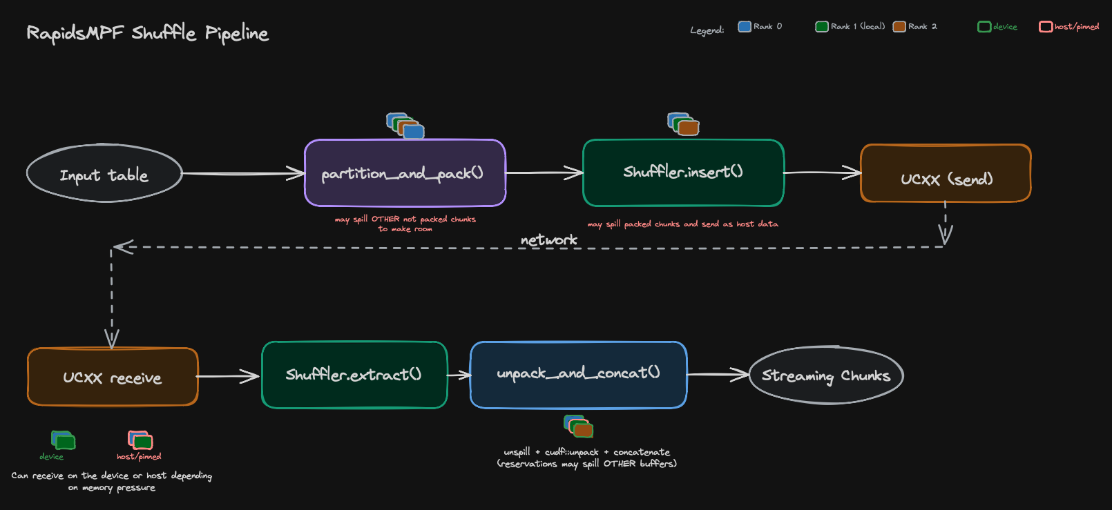
Interesting! Global throughput has degraded substantially, to ~480 GiB/s and we have two new lines in the statistics: alloc-pinned_host and copy-pinned_host-to-device -- but we don't see any line like copy-device-to-pinned_host. That absence is the interesting part. We are still shuffling the same amount of data: each rank has 20GiBs, they receive 17.5GiBs from the other 7 ranks; at a limit of 32GBs, each rank is now over the limit. However! As RapidsMPF is moving data around, the receive side can observe the memory pressure and knows about the configured device limit. Instead of thrashing and moving data back and forth several times D->H/H->D/and back again, the receive side can accept buffers on the host instead of the device to avoid the thrashing -- thanks UCXX!

In other words, nothing was evicted from the device; the data simply never landed there in the first place. Spilling that never has to spill is the cheapest kind.

Why such a big performance hit? Of the reported 335.15 ms, RapidsMPF is spending 171.8 ms moving data back to the device.

copy-pinned_host-to-device: 5.62 GiB | 171.80 ms | 32.74 GiB/s | avg-stream-delay 1.78 ms

The DGXB200 has PCIe Gen 5 which has a transfer rate of 64 GB/s for all 16 lanes. RapidsMPF is moving data across this bus at an average rate of 32 GiB/s per GPU. These shuffles are using pinned memory and still, it's a bottleneck for spilling. If we swapped out the x86 chips and used a Grace-Blackwell configuration with C2C we could easily 5x-10x the bandwidth between host and device. C2C can transfer at up to 900 GB/s.

Below is a table sweeping the same initial setup while ratcheting the device memory limit down and correspondingly, the memory pressure also increases forcing more spilling to occur:

Scaled Spilling DGXB200¶

Label	Spill limit	Peak device	Local perf	Global throughput	D2H (pinned) vol / time / rate	H2D (pinned) vol / time / rate
no-spill	∞ GiB	60.0 GiB	229.7 GiB/s	1.79 TiB/s	0	0
onset-spill	32 GiB	60.0 GiB	60.0 GiB/s	480.2 GiB/s	0	5.6 GiB / 191.4 ms / 29.4 GiB/s
light-spill	28 GiB	60.0 GiB	35.9 GiB/s	287.0 GiB/s	0	9.7 GiB / 379.0 ms / 25.6 GiB/s
moderate-spill	24 GiB	60.0 GiB	26.5 GiB/s	211.7 GiB/s	0	13.8 GiB / 491.0 ms / 28.0 GiB/s
heavy-spill	20 GiB	60.0 GiB	14.8 GiB/s	118.6 GiB/s	0.3 GiB / 9.6 ms / 32.6 GiB/s	17.5 GiB / 622.3 ms / 28.1 GiB/s
very-heavy-spill	16 GiB	60.0 GiB	10.1 GiB/s	80.5 GiB/s	4.1 GiB / 128.7 ms / 31.6 GiB/s	18.1 GiB / 1340.0 ms / 13.5 GiB/s
extreme-spill	12 GiB	60.0 GiB	6.9 GiB/s	55.5 GiB/s	8.1 GiB / 264.5 ms / 30.7 GiB/s	18.8 GiB / 1170.0 ms / 16.1 GiB/s

A note on how to read the table: the throughput columns are rank 0, while the spill volumes and times are the worst-case rank of the eight, since that's the one you actually wait for. Raw logs and run scripts are in scaled-spilling-b200 if you want to explore further.

Reading down the table, a few things stand out:

The degradation is smooth and monotonic. As we lower the device memory limit we are going to be spending more time moving data back and forth between host and device at PCIe Gen 5 speed, but importantly it does not OOM.
Receive-side mechanics can avoid pointless thrashing copy-device-to-pinned_host is 0 for the first four spill levels and RapidsMPF never evicts anything, receiving incoming buffers on the host to mitigate the device memory limit we imposed. Only at a 20 GiB limit, where the limit equals the input size, does real device-to-host spilling kick in.
Spilling is the expensive part. copy-pinned_host-to-device climbs from 5.6 GiB to 18.8 GiB, and the time to move it grows from 191 ms to 1170 ms. The transfer rate between host and device though is mitigated with pinned memory buffers (as we've discussed before). If we changed the hardware and used C2C with 900 GB/s of bandwidth, we would be much better off.

Wrapping Up¶

I think we've sufficiently demonstrated how challenging and memory intensive shuffles (and the implied joins, sorts, etc) can be. Unconstrained, RapidsMPF drives roughly 1.8 TiB/s of global throughput on a DGX B200. Perhaps more importantly RapidsMPF can successfully shuffle without needless thrashing and OOMing while leveraging accelerated transport when shuffling. And not only that, we have hardware solutions already in place to alleviate the choke points of bandwidth between host and device transfers.

Recall the challenges of shuffles: Memory Intensive, Transport, Synchronization. RapidsMPF mitigates these problems:

Memory intensive: RapidsMPF can spill/evict buffers from the device at tunable limits AND can receive bytes on the host to prevent unnecessary thrashing.
Transport: RapidsMPF utilizes UCXX which enables transport across NVLink, InfiniBand, EFA, TCP, etc.
Synchronization: RapidsMPF addresses this challenge with an asynchronous/streaming execution model that overlaps the shuffle with other ready work. In a follow-up post we'll get into these details.

We set out wanting a shuffle that is fast, scales, and handles larger-than-VRAM data and we have that with RapidsMPF. Users can reuse this library directly, or implement these ideas in their own projects.

In a later post we'll return to studying scaling on an NVL72 -- get ready for some weak and strong plots!